In previous articles, I stated that I wrote a computer program to work out the math for my analyses, the Magic Probability Toolkit. While I have made the source code for the Toolkit available, several people asked that I go one step further. They requested more detail on how the Toolkit works. What are the steps it takes to get me my results? Could you please explain the math behind the numbers?
Thus far I’ve shied away from getting into the nitty-gritty, as it is not my intent to drown people in a flood of mathematical details. In general, I want to write articles that can be consumed casually and which do not require a calculator to understand. At its core, the Magic Probability Toolkit is quite simple really—just a probabilistic application of dragscoop ionics and electropropulsion magnetronics.
But apparently Izzet readers hunger for more detail than that. This article is for those readers. The ones who want to dive a little bit deeper into the math. This article does not offer up insights into the game of Magic. Rather, its insights are into the math of probability and the inner workings of my Toolkit. Hopefully, understanding my methods will allow you to better appreciate the results in the previous and future Limiting Chance articles. But if that doesn’t sound like your cup of tea, don’t worry. The enjoyment and understanding of future articles will not be contingent on the reading of this one.
Calculating Probability
The foundation of my articles is the ability to calculate the probability of an event occurring in a game of Magic. There are three basic ways to determine the probability of an event no matter what the field of study:
- Physically measure the probability.
- Use Monte Carlo methods to numerically sample a large (but incomplete) set of possible outcomes.
- Solve for the exact closed-form solution.
Each option has its pros and cons. Which one is appropriate depends on the characteristics of the system you are analyzing.
Physical Measurement
By this I mean literally sitting down and performing the action a large number of times. Write down what happens each time. Take the number of times the event occurred, divide it by the number of times I performed the action, and that is my probability.
If I am trying to determine the probability of drawing three lands in an opening hand of seven cards, that means I shuffle, draw seven cards, and record whether or not I drew three lands. Then I shuffle again, draw seven cards, record the result, shuffle, draw seven cards, record, etc. I repeat those steps a large number of times. The number of times I draw three lands divided by the number of times I repeat the steps is my probability measurement.
If I want to make sure my measurement is accurate, I repeat the entire process a few times, each time performing the same large number of shuffles and draws. Then I compare the results. I’ll get a slightly different answer each time, but if all of the answers are close together, I can be fairly sure that my result is close to the true probability. The more times I shuffled that deck, the more accurate my result will be.
Based on the fact that this approach involves reshuffling a deck over and over again, it’s pretty clear that the method is not so hot for Magic. (Although in truth, this is exactly how all of us develop an intuition for Magic probabilities. We just play tons and tons of Magic, slowly reducing the error on our mental probability measurements until we’re good players.) So when is this method useful? It’s great for experimental science, where you don’t often understand the mechanisms that are operating behind the scenes to determine if the event occurs. This method is basically just the same thing as "doing an experiment."
Monte Carlo
Monte Carlo is the name of a category of computer algorithms that use random sampling to compute results. The technique can be used to calculate a number of different things, including probability. Using Monte Carlo to compute probability is quite similar to doing a physical measurement, but instead of performing the action yourself, you let a computer do the work.
Let’s stick with the example from before where I am determining the probability of drawing three land in a seven-card hand. To calculate the probability using Monte Carlo, I write a computer program that keeps track of the order of cards in a deck. That deck lives only in the memory of my computer. I write an algorithm that randomizes the order of the cards, effectively shuffling the deck. After shuffling the deck, I have the computer check the top seven cards and record whether three of them are lands. Finally, I have the computer repeat the process a large number of times, and I have my answer.
Assuming I can code the program faster than I can repeatedly shuffle a 40-card deck, I’ve saved time! Plus now that I have the program written, I can probably use it to do other analyses, like determining the probably of drawing two lands in a seven-card hand.
When is Monte Carlo the right approach to calculate a probability? It’s the right approach when both of the following are true.
- The process under analysis has an extremely large number of possible outcomes, a number is so large that even a computer cannot look at every single outcome in a reasonable amount of time. If the number of outcomes is not that large, the closed-form approach described in the next section should be used instead.
- The mechanisms governing the process are understood and can be programmed into a computer. As such, Monte Carlo cannot be used in place of physical measurement in scientific pursuits where the physical mechanisms are not understood.
Monte Carlo is potentially a useful approach for Magic. Having a computer shuffle a digital deck is obviously preferable to shuffling a physical deck a huge number of times. And coding up the mechanisms governing Magic is not a problem because we know the rules of the game.
However, Monte Carlo is not the technique used by the Magic Probability Toolkit. The questions I have confronted so far have not had a large enough number of possible outcomes, at least not large enough to warrant using Monte Carlo. For example, if I only care whether or not a card is a land or a spell (ignoring everything else about the card such as color, casting cost, etc.) and assuming I care about the order of the draws, the number of possible outcomes when I draw seven cards is 128. That’s two to the power of seven; seven instances in which one of two things can occur. With only 128 possible outcomes, a computer can easily investigate all possible outcomes in a short period of time. There is no sense in using Monte Carlo.
However, let’s kick things up a notch. Perhaps I am doing an analysis which does require me to consider the color and casting cost of spells. An example of such an analysis might be one where I am trying to calculate the "perfect" mana curve for a two-color deck. Let’s say I have to consider every spell as unique in a 23-spell deck. There are no longer only two outcomes to each draw (land or spell). There are now 25 different outcomes to each draw (23 spells plus two land types). The count of all possible outcomes is now 25 (instead of two) to the power of seven, or about 6,100,000,000.
(Veterans of probability and combinatorics might point out that the count is actually somewhere between that number and a smaller, but still very large, number equal to 25! ÷ 18!. Why not exactly 25! ÷ 18!, they might ask? Because when you draw a basic land, it doesn’t eliminate one of the possible outcomes for future draws. The basic lands complicate the calculation.)
(Another thing that might trouble advanced readers is why I insist on caring about the order of the draws. Caring about the order significantly increases the number of possible outcomes. Such readers might point out that the order of the draws in the opening hand is unimportant. However, once I move past the opening hand and analyze draws that occur during game play, the order becomes very important. Thus it is not unreasonable to consider draw order when speaking roughly about the number of possible outcomes that could be under analysis.)
The number 6,100,000,000 is very large. Once you move past the opening hand and into a full game of Magic, which might last twelve or more turns, the numbers become even larger. Just as an example, the count of possible card orders that a 40-card deck can have after shuffling is 40!, or an eight with 47 zeros after it. I think it’s pretty likely that I will find myself coding up a Monte Carlo algorithm sometime in the future.
Closed Form
Solving for probability in closed form basically means figuring out an equation that gives the exact value for the probability. There is no measurement, no estimations of error—just math.
For very simple cases, "figuring out" the equation can be as simple as thinking about it for a fraction of a second. What’s probability of getting heads when I flip a coin? There are two possible outcomes, so one in two, or 50% of course. The more experience a person has with probability, the more likely they are to know the formula for a situation. For example the formula for the probability of drawing a certain number of lands in my opening hand is this:
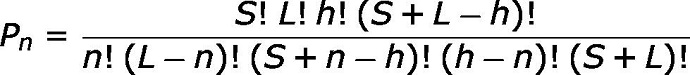
Here L is the number of lands in my deck, S is the number of spells in my deck, h is the number of cards in my hand, and n is the number of lands in my hand. If I punch in the numbers for a three-land hand (L = 17, S = 23, h = 7, n = 3), I get 32.3%. (Check back to the first article in the series and you’ll see that the result matches my table.) That formula is called the hypergeometric distribution function. You may have seen it mentioned in the comments.
Knowing the probability formula for a large number of situations is very useful, but no matter how many formula you know, you’ll eventually run across a problem you don’t know the formula for. That is when you have to derive the formula from first principles. (In fact, that is probably how Leonhard Euler first worked out the hypergeometric distribution back in the 1700s.)
So how do you derive a probability from first principles? There are a number of approaches. Here is one of the most straightforward ones.
If I have a series of actions I am going to take and those actions can result is a number of different outcomes, I can determine the probability of obtaining a favorable outcome using the following steps. (By "favorable outcome" I simply mean that the outcome matches whatever it is that I am trying to measure the probability of.)
- List all possible outcomes.
- Identify which of those outcomes are favorable.
- Break down each outcome into a set of simple, independent events; events so simple that the probability of them individually is obvious.
- For each outcome, multiply the probability of the independent events to determine the probability of the outcome.
- Sum the probability of all favorable outcomes.
To illustrate the steps, let’s walk through a simple example.
Say I have a card game with a deck of ten cards, and each card represents a building resource. Five of the cards are wood, three are clay, and two are stone. I want to determine the probability of getting at least one wood and one stone when I draw three cards at random.
(Readers experienced in combinatorics might point out that this example is simple enough that there is actually a known formula for it. In this case it’s called the multivariate hypergeometric distribution function. But that is not the point. The point is to use a relatively simple example so that the underlying theory becomes clear.)
First, I list all possible outcomes. For each of my three draws, I can draw any of the three resources. If I list out all of the possible draws that could happen, I get a list of 27 outcomes. That’s three (the number of draws) to the power of three (the number of card types). Here’s the list, with the three cards listed in the order they are drawn, using W for a wood card, C for clay, and S for stone.
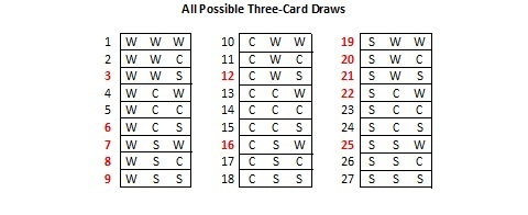
Now I identify which outcomes are favorable. Favorable means that they match what I am calculating the probability of. It means that the draw includes at least one wood (W) and one stone (S). I’ve colored red the outcomes in the chart that are favorable: outcomes 3, 6, 7, 8, 9, 12, 16, 19, 20, 21, 22, and 25.
Then I break each outcome down into a set of simple events. Drawing a single card is a simple event. I know the probably of drawing a card if I know what is in the deck. So I break down each outcome into three independent draws. The probability of the outcome as a whole is obtained by multiplying the probability of the three smaller events, the three draws.
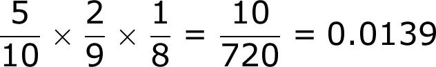
Let’s work through one of the outcomes explicitly. We’ll do outcome number 9. In that outcome I draw a wood first, then a stone, then another stone. Figuring out the probability of each draw is easy. It’s the amount of that resource left in the deck divided by the number of cards left in the deck. The chance of drawing wood is five in ten. After that, the chance of drawing stone is two in nine, and the chance of drawing another stone is one in eight. I multiply those together to get the overall probability of the outcome.
Here is a complete table of probabilities for the favorable outcomes.

I add those all up, and I get the total probability of drawing at least one wood and one stone in three draws: 45.8%. There, I’ve done it! I’ve calculated the probability in closed form.
What a pain.
Magic Probability Toolkit
The Magic Probability Toolkit uses that sort of first principles approach to generate closed-form solutions. It performs the same basic steps described in the previous section but organizes those steps somewhat differently. It organizes the steps in a way that makes it easier for the user to think about the problem in terms of actions that occur in a game of Magic.
The fundamental data structure used by the Toolkit is a list of data blocks. Each data block holds the state of a game of Magic. The amount of detail used to describe the state of the game depends on the complexity of the analysis. In the simplest analyses, the state tracks the number of spells in a player’s hand, the number of lands in the player’s hand, and the number of spells and lands in the player’s library.
Each data block also holds a probability for its state. The sum of all probabilities in the list adds up to 100%. The list of states can be thought of as a probability distribution of a game of Magic. It answers the questions: what possible states can the game be in and what are the probabilities of those states?
At the start of each calculation, only one state is in the list. That is the initial state of the game, and it has a probability of 100%. As an example, let’s look at a calculation about a player who starts the game with a three-land hand. At the beginning of the calculation, the single state in the probability distribution is:

(It’s worth noting that the Toolkit also supports more complex states. For example, a more complex analysis might use states that hold information about the library and hand of both players. Or the states might track additional details about the cards, such as land type or spell color. For this illustration, however, I’ll keep it simple.)
Once the initial state list is setup, I can take actions in the game that cause the probability distribution to evolve forward. For example, I can have the player draw a card. The Toolkit will advance the state list forward to exhibit all possible states after the draw. The probability distribution then looks like this.
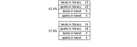
If I tell the Toolkit to have the player draw another card, it will go through the state list and replace each state with all possible results of drawing a card while in that state. The probability of a replaced state is distributed among the states it creates based on the relative chance the new states have of occurring. The Toolkit also merges all equivalent states after performing an action, summing their probabilities. So during a second card draw, the two states split into four states. Two of those four are equivalent, so those two then merge and we are left with a three-state probability distribution that looks like this.

The state list is now two draws into the game of Magic. You can think of each state as a possible future for the game at turn two. The probability of each state corresponds to the likelihood of that future coming to pass.
Actions
The Toolkit currently has support for these game actions.
- Draw a card.
- Draw a card if a condition is true.
- Draw cards until a condition is true.
- Mulligan if a condition is true.
With the second and subsequent actions, some states will meet the condition and some states will not. It is the existence of these conditional actions that takes the Toolkit beyond the domain of the multivariate hypergeometric distribution.
The mulligan is a particularly complex action, as it breaks a single state down into a large number of future states: one for each hand that the mulligan could result in.
Measurements
Once all of the actions that an analysis calls for have been applied to the probability distribution, I can use the Toolkit to perform measurements on the game’s possible futures. These measurements take one of two forms.
- Calculating the probability of something occurring.
- Calculating the average value of some quantity.
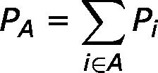
Calculating the probability of some condition occurring is straightforward. The Toolkit sums the probability of all states in which that condition is true. For example, perhaps I want to measure the probably that the player has more spells than lands in his hand. The Toolkit simply checks each state to see if that condition is true for the state and, if so, adds it to a running sum. The procedure can be summarized with the following formula, where Pi is the probability of state i, and A is the set of all states that match the condition.
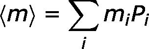
Calculating the average value of a quantity is only slightly more complex. An example of an average value that I might want to calculate is: how many more spells, on average, does my opponent have in his hand than I do in mine? This sort of measurement is performed by taking a weighted average of that quantity across all states. The Toolkit calculates the value of the quantity in each state, multiplies that value by the probability of the state, and sums the results. That procedure can be summarized with the following formula, where mi is the value of the quantity in state i, and Pi is the probability of state i. Here the sum is over all states.
Download
That’s about all there is to know about the mathematical methods I use for my articles. Hopefully this background will cause a few more people to download the Toolkit and give it a try. If you want any more detail on how things work, downloading it and taking a look at the source is definitely the way to go.
As I write articles, my plan is to extend the functionality of the Toolkit. At a minimum, new versions will be posted with each article containing the analysis for that and all previous articles. Give it a try!
[email protected]
@DanRLN on Twitter
source code for the Magic Probability Toolkit
 |
I’m with the Simic Combine. I’m a scientist, but I’m also a lover of nature. Plus, enemy color combinations always produce more interesting spells, and of all enemy colors, blue-green has the smallest overlap in both abilities and flavor. So blue-green cards are always crazy awesome! I mean, come on. Mystic Snake! |